QUBO Solving ASIC

What is QUBO?

QUBO stands for Quadrature Unconstrained Binary Optimization. It’s an unconstrained discrete optimization problem.

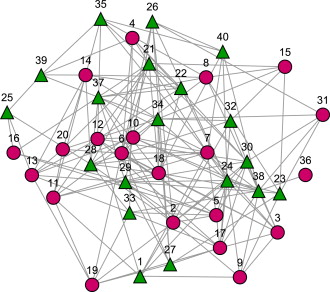
The problem goes like this:

• We’re given an $n \times n$ matrix $Q$ that encodes the weights of a min/max problem
  • This problem can usually be represented as a graph with nodes A,B,C… and weights $N_{1}$, $N_{2}$… across each node
  • Keep in mind that obtaining the $Q$ matrix from a graph problem is itself a tricky problem. Usually the problems involve the relationship between nodes, themselves, and their neighbors, so we can usually represent “self weights” in the diagonal, and “relationship weights” in the non-diagonal. This may not always be the case.
  • For the rest of the project, we should assume we already have a correct $Q$
  • $Q$ is usually symmetrical
• We are trying to solve $\text{argmin}_{x}(x^T Qx)$
  • $x$ is an n x 1 column vector that represents the “binary solutions” of QUBO. $x_{i} \in {0,1}$
    • In the problem, $x$ usually describes an optimal combination of weights in the graph. Because these are “presence of weights,” they are usually a 1 or 0, as in no presence or all presence. This is where “binary” comes in.
• So we go from a matrix, to a minimization of an equation. This is the “cost function” that we are minimizing.
  • You can check that the result of $x^T Q x$ is a scalar and not a vector or matrix

We can relate the QUBO problem to the Ising Hamiltonian for a Quantum system

• The ISING Hamiltonian represents the energy state of $N$ electrons with spins. A spin can be either a +1 (up spin) or -1 (down spin).
  • $H(s) = C+h^Ts + \frac{1}{2} s^TJs$
    • $s$ is an n x 1 vector representing the spin states of all electrons
    • $h$ is a vector of “external magnetic fields” that can influence the strength of each individual spin
    • $J$ is a matrix that encodes interactions between different spins. For example, spin 1 and spin 2 can have a relationship $J_{12}$.
  • $H(s)$ describes the energy state of the system with N electrons, each with a +1 or -1 spin
    • $H(s)$ wants to be minimized such that the system can be at its lowest energy state. That means each electron should be configured in its OPTIMAL SPIN STATE such that the system has the least energy.
• You may notice that the Ising Hamiltonian and the QUBO $\text{argmin}$ have very similar forms.
  • In fact, they’re exactly mappable onto each other.
  • The important part is that they’re both binary optimization functions that input matrix problems and output vector solutions. For QUBO, the solution is a vector of binary values representing weights that minimize the cost function. For the Ising Hamiltonian, the solution is a vector of +1 or -1 representing the spins of the electrons such that the system has least energy.
• In fact, the QUBO argmin and the Ising hamiltonian are exactly related by the relationship $s = \frac{x+1}{2}$
  • The above relationship turns a QUBO binary into a spin state in the Ising Hamiltonian
  • If you substitute $x$ for $s$ with that relationship, you get a solution exactly in the form of the Ising Hamiltonian

Relationships:

• $h = \frac{1}{2}Q (1)$
• $J = \frac{1}{2}Q$ with no diagonals.
• So we can construct $H(s) = h^Ts + \frac{1}{2}s^TJs$ from just $Q$
• Note that these relationships will be used to make some clever shortcuts later.

Simulated Annealing

To summarize from the previous part:

• QUBO Problem → Q matrix → $\text{argmin}_{x}(x^T Qx)$ → $\text{argmin}_{s}(H(s))$

We now have an evaluation function $H(s)$ that inputs a proposed solution $s$ and outputs energy $H(s)$. These are all the building blocks you need for meta-heuristic optimization.

Why Simulated Annealing?

• For a greedy algorithm like gradient descent, you choose the path of least resistance 100% of the time. As in, you always “follow the gradient.” This is great for convex and convex-like problems because you always know that the local minimum is also the global minimum.
• But for many discrete optimization problems, the energy landscape is somewhat more complicated, and gets much more complicated the larger the dataset is. Therefore, greedy methods like gradient descent will fail to capture the global minimum (or even an approximate global minimum) almost 100% of the time.
• This is where meta-heuristic methods become advantageous. The central premise of this is:
  • You will lose the deterministic time complexity. In exchange, you get a probabilistic advantage by strategically inserting randomness.
  • Simulated Annealing is a meta-heuristic that bets on “probabilistic convergence.” As in, the acceptance of non-greedy steps follows a converging probabilistic model. You are therefore more likely to find the global solution because you cover more of the solution space by allowing non-greedy steps.
• In the world of meta-heuristics, time complexity is thrown out the window. Instead, the benchmark is time.

So how does Simulated Annealing work?

• We start with a randomized solution $s_{0}$. We can evaluate this solution with $H(s_{0}) = H_{0}$. These are the initial variables.
• $\alpha$ is the cooling rate, which can be tuned.
• Loop:
  • Start
  • Randomize one of the spin states of $s_{0}$ to make $s_{1}$. Then find $\nabla H = H_{1} -H_{0}$
  • If $\nabla H \le 0$, accept the spin change
  • If $\nabla H>0$, conditionally accept the spin change according to the model $P = e^{-\alpha\cdot\nabla H/T}$ where $T$ is the “temperature” of the loop at a given step
  • $T_{new} = T_{old} \cdot \alpha$
  • End
• At the end of the loop, the temperature will have gone down to a threshold $T_{min}$.

This is the algorithm we’ll be using, the algorithm at the core of the computation.

Verilog Implementation

The starting implementation will be a random 5 x 5 Q matrix, representing an arbitrary QUBO problem. We can assume the Q matrix is diagonal and correctly encodes the QUBO weights and correlations. The entries in the matrix are whole integers that can be negative, positive, or zero, and can go up to the value 32.

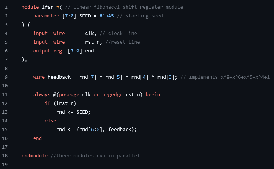
The “stochasticity” of this stochastic optimizer comes from a random number generator. Specifically, it uses a Fibonacci LFSR, an X-bit long register with a Y-bit long XOR operation that supplies the next bit value after shifting a register to the left.

From a starting seed (input of bits in the register), the LFSR can generate a cyclical random sequence of bits. Most importantly, it will never get stuck. For this implementation, it uses an 8-bit LFSR with a 4-bit input XOR. This can generate a random bit cycle of length 255, before repeating its values, meaning it will take 255 clock cycles before the output starts becoming deterministic. Thus, it is not a truly random number generator. The width of the LFSR can increase to exponentially increase the # of clock cycles, which can, in practice, make this a random number generator.

The output of the LFSR supplies both the spin update (spin flip operation) and the Metropolis test (probabilistic choice after checking if the energy is lower).

Let’s start with some instantiation.

• 15-signed Q-port inputs create a 5 x 5 upper triangular matrix. Because the $Q$ matrix is diagonal, we can be more storage efficient by only storing the upper triangular.
• We set the number of temperature steps, the four states [S_IDLE], [S_RUN], [S_COOL], [S_DONE], and the register to store the states for updates in the FSM. We create $q_{00} \dots q_{{44}}$ as part of storage to compute $h_{0} \dots h_{4}$ (remember $h$ is part of the Ising Hamiltonian).
• We instantiate the spin register to store our solution, temperature register (16-bit integer), attempt count, and temperature count. Let’s compute $h_{0} \dots h_{4}$ with a wire assignment $h_{0} = 2 \cdot q_{00} + q_{01} + q_{02} + q_{03} + q_{04}$, etc. Again, we know how to compute $h_{i}$ because of the relationship between the Ising Hamiltonian and the QUBO $\text{argmin x}$ formulation (which was given earlier). $h$ can be computed as a row product of $Q$. This means we don’t have to completely recompute $H(s)$ every loop, which would be computationally wasteful.

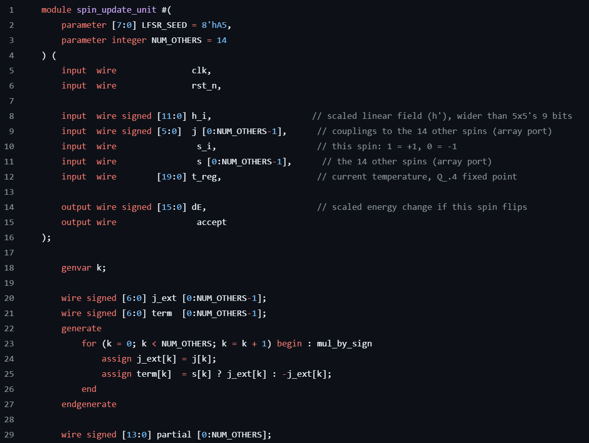
Next we start doing spin updates.

• We have 5 spin update module instantiations in parallel, each one gets its own $h_{i}$, 4 couplings, 4 views of other spins, and a distinct LFSR seed for random number generation. Because this is hardware implemented, we can have as many spin updates in parallel as we like, we’re not sequentially limited or limited by the number of cores.
• In theory, this could scale as much as can fit on a chip, which would drastically improve the convergence rate of the optimizer.

Next we do temperature cooling.

• We multiply the temperature by a fixed α cooling rate, represented by a 24-bit integer. We can tune the cooling rate according to performance. This is the only place on the chip where any integer is actually multiplied.
• This loop then goes back to the previous loop, or to the final loop where the output is given as $x_{out}$.

Notice that we don’t compute a new $x^TQx$ or a $H(s)$ every time. We want to avoid computationally expensive operations wherever we can, and we can in this case by finding the relationship between the Ising Hamiltonian and the QUBO Argmin. That relationship turns out to be a few linear relationships that don’t even involve integer or matrix multiplication. That is huge!

Performance Benchmarks

Input: $5 \times 5$ Q Matrix

• q00 = -27, q01 = 22, q02 = -27, q03 = 12, q04 = -20
• q11 = 17, q12 = -26, q13 = 1, q14 = 30
• q22 = 9, q23 = 15, q24 = 16
• q33 = -4, q34 = 13
• q44 =-5

Initial Solution Vector:

• {1,1,1,1,1}

Results:

Stochastic Optimizer (Simulated Annealing)

• Cycles #: 441 (4410 ns)

Brute Force (Linear best search)

• Cycles #: 33 (330 ns)

Optimized Solution Vector (both methods match):

• {1,0,1,0,1}

On average, the optimizer reached the solution after 4410 ns. The total # of spin flips during the run was 186. The final solution was {1,0,1,0,1}. The brute force approach also reached the final solution {1,0,1,0,1}.

In this case, the brute force solution was 13.4x faster. This makes sense, the solution space is only an 8-bit integer. So you may be wondering why we’re taking so much extra effort when even a brute force search was faster.

Now let’s make some changes. We’ll change our scale to a $Q$ matrix of $15 \times 15$ (we’re just adapting the $5 \times 5$ case to the new case, not changing any core computation), and compare the Simulated Annealing algorithm vs. the Brute Force approach.

Input: $15 \times 15$ Q matrix

• 28,20,-24,19,-25,-3,20,-13,-11,-15,14,-16,31,-4,-2
• 20,8,0,5,3,0,31,19,18,12,7,-11,31,-3,-19
• -24,0,11,22,-22,22,7,-25,-30,-4,-30,-23,0,30,-3
• 19,5,22,25,19,26,20,8,-4,0,-15,-1,-8,-17,31
• -25,3,-22,19,5,-32,-26,-20,30,12,24,-20,14,-9,-1
• -3,0,22,26,-32,17,-32,7,21,10,-23,2,-15,29,24
• 20,31,7,20,-26,-32,21,-21,0,28,22,13,8,-30,15
• -13,19,-25,8,-20,7,-21,-18,-2,-27,-17,2,14,0,7
• -11,18,-30,-4,30,21,0,-2,-29,23,11,-9,9,6,-26
• -15,12,-4,0,12,10,28,-27,23,-13,-29,10,-8,6,-12
• 14,7,-30,-15,24,-23,22,-17,11,-29,-14,-18,-23,-8,20
• -16,-11,-23,-1,-20,2,13,2,-9,10,-18,23,-7,-8,4
• 31,31,0,-8,14,-15,8,14,9,-8,-23,-7,26,30,-7
• -4,-3,30,-17,-9,29,-30,0,6,6,-8,-8,30,-32,5
• -2,-19,-3,31,-1,24,15,7,-26,-12,20,4,-7,5,-1

Initial Solution Vector:

• {0,0,0,0,0,0,0,0,0,0,0,0,0,0,0}

Results:

Stochastic Optimizer (Simulated Annealing)

• Cycles #: 441 (4410 ns)

Brute Force (Linear best search)

• Cycles #: 32769 (32769 ns)

Optimized Solution Vector (both methods match):

• {1,1,0,1,1,1,1,1,0,0,1,0,1,0,1}

On average, the optimizer reached the optimal solution after 4410 ns. The total # of spin flips during the run was 169. If you noticed, the convergence time was actually the same as the previous $5 \times 5$ case. This is because I didn’t change the convergence runtime for the Simulated Annealing algorithm, meaning all the parameters were actually the same as the $5 \times 5$ version (it ran for the same # of total steps). And look at that, it still converged.

In this case, the simulated annealing solution was 74.3x faster. The search space for the brute force method exponentially scales to a linearly scaling increase in size, $O\log(2^n)$.

Keep in mind, this is before tuning and optimization. We could tune the initial solution vector to start at a more advantageous position to converge faster. We could tune the temperature cooling rate to the problem by perturbing and seeing which direction goes faster. We could also stack more compute modules in parallel.

Now for the final change. Let’s move to a $30 \times 30$ Q matrix. At this point and beyond, brute force solutions become impractical. An exhausting search would take 1.07 billion steps, which is a complete waste of computational resources. Now we have to evaluate in the dark.

Input: (I’m not pasting the whole matrix)

Initial Solution Vector:

• {0,0,0,0,0,0,0,0,0,0,0,0,0,0,0,0,0,0,0,0,0,0,0,0,0,0,0,0,0,0}

Stochastic Optimizer (Simulated Annealing)

• Convergence time: 4410 ns (this parameter didn’t change)

Optimized Solution Vector:

• {1,1,0,1,1,1,1,1,1,0,0,1,1,1,0,1,1,1,1,0,0,1,1,0,1,1,1,1,1,0}

So how do we know if this is the optimal solution vector? Well, we don’t. But we can try to see if we can find a better one by running the algorithm for longer.

Let’s extend the length of the algorithm by double to see what we get:

Initial Solution Vector:

• {0,0,0,0,0,0,0,0,0,0,0,0,0,0,0,0,0,0,0,0,0,0,0,0,0,0,0,0,0,0}

Stochastic Optimizer (Simulated Annealing)

• Convergence time: 8410 ns (roughly double from before)
• Accepted flips: 328 (compared to 190)

Optimized Solution Vector:

• {1,1,0,1,1,1,1,1,1,0,0,1,1,1,0,1,1,1,1,0,0,1,1,0,1,1,1,1,1,0}

I’ll save you the time that it takes to check if the solutions are the same. They are. So it looks like the initial convergence is actually optimal (comparing with a longer-running algorithm). So assuming that the solution is at the global minimum (or close), the convergence rate is extremely fast and scales slower than the matrix size increase.

In the future, I will do a schematic level review and layout for hardware. This is the part I’m most excited about.

You can find the repo here: QUBO Solver Verilog Implementation