Digital Towed Array
signal-processingacousticsTinyML
This article includes research done in collaboration by me and Supun Randeni. Much of the content here will be included in a paper publishing in the Fall of 2027.
A Towed Array is a long array of sensors that gets dragged behind large vessels at sea (ships, submarines). Its primary purpose is to detect the presence of a particular signal, and find what direction it’s coming from. In submarines for example, a towed array is used to detect the presence of other submarines.
The standard towed array architecture is a series of hydrophones (piezo-electric transducers with a pre-amp) connected to a multiplexed data bus, which is connected to a vehicle. The vehicle takes waveform information from the hydrophones and beamforms. The vehicle then runs a “beamforming algorithm,” which allows the system to determine which direction the signal is coming from.
The beamforming algorithm looks like this:
For an N-th node receiving a signal where it can be in the form:
Each node N sees this:
- is the received signal by the -th array
- is a phase delay
- is noise
Phase-Adjust:
Sum the signals:
- where is a weight for the th node signal
Propagation delay is defined by:
- Relative to the first sensor:
Array response for direction
Power transmitted from direction :
- is the Hermitian transpose of the array response
- Basically a transpose but you also take the complex conjugate of each element
- is the vector of all the responses for every node
Then find the sum of all power transmitted omni-directionally
- ,
- where is the total amount of samples across the azimuth
Basically, by computing the energy from an omni-directional sample, we can find the direction that a signal comes from by finding the direction that has the most energy. This is the essential formula for beamforming.
From Analog to Digital Towed Array (DTA)
This research investigates the potential of a new architecture proposed by us: by offloading compute from the vehicle to each node in the array, we can reap a number of benefits.
- Lower latency
- By processing the signal per node and returning the output to the master, we can increase the speed of beamforming.
- Parallel processing
- Each node processes its data in parallel rather than the vehicle processing the data sequentially.
- Simplified data bus architecture
- Instead of feeding all of the waveform information to the vehicle from each node, we can process the waveforms on the node, and output much simpler data to the master.
- Synergy with Deep Neural Networks
- Each node can run its own classifier neural network, with its own weights from training. We can take advantage of the system’s parallelism to synergize with the parallelism from training a Multi-Layer Perceptron (MLP).
In order to do this, we have to switch from a traditional beamforming architecture to a “distributed” beamforming architecture. We can do this because, in order to beamform, all we need are two pieces of information:
- Amplitude of the signals relative to each other
- Phase of the signals relative to each other
Distributed beamforming techniques have been described before in previous papers, mostly in drone localization research. In those papers, each drone acts like a “node” in a distributed array, and each drone processes signal data and passes them to other drones.
In the Digital Towed Array, each node acts as its own localized compute, and communicates beamforming information to the master. Each node cannot beamform because beamforming requires information from every node at once, and it’s easiest to send all of the beamforming information to a controller.
Hardware Architecture
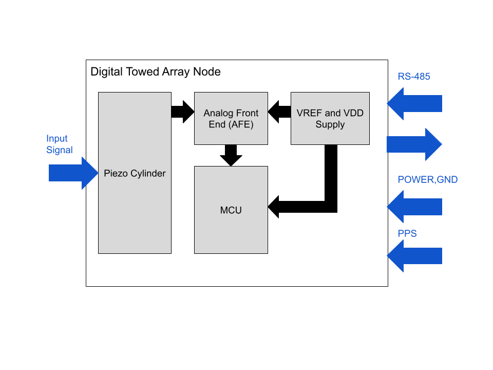
Each node has an STM32G431 as its local compute, and uses its ADC. It communicates to the master through RS-485, and the data bus gets sent down the entire line. We use a charge amplifier at the pre-amp to condition the signal from a piezo-electric cylinder (which acts as a capacitive element). A power bus +5V and GND runs through the whole towed array.
A differential PPS line (pulse-per-second) acts as a ground truth clock, and synchronizes every node with the vehicle’s clock. This synchronization is critical for beamforming because we need to preserve precise time information. Otherwise, beamforming is impossible.
From Digital to Smart Towed Array (STA)
One of the unique benefits of the Digital Towed Array architecture is the ability to put a classifier neural network on each node. There are many benefits to this:
- Parallelism
- We can offload compute from the vehicle to the nodes, making processing faster.
- Training Diversity
- Each node gets trained independently from each other, so each node has its own parameters . This increases the training diversity in the total neural network. We can also choose to re-use the parameters.
- “Group Huddle” Aggregation
- Each node can output a one-hot encoding of its proposed solution. So even if one node or multiple nodes get the answer wrong, as long as the majority of the nodes agree on the correct answer, the system can classify correctly. This makes the Smart Towed Array more immune to disruptions from noise from the input signal. We’ll demonstrate the effectiveness of this approach later.
Furthermore, our data is relatively simple to process, giving it an advantage in speed.
- Each node needs to process , which can be encoded as an vector . We can then run through a DNN.
Let’s explain this method using a simpler example: a waveform classifier. We’ll run through the interpretation, and then an example in python. Then we’ll try to fit it on the STM32G431 that we’re using. The general architecture of this simple example is broadly applicable to any input signals that we want to classify, which is why it’s useful to map out now.
Example: we want to classify three types of waveforms from input data: sine waves, square waves, and sawtooth waves.
- Our input is a vector that encodes the input signal from the analog front end. In this example, we’re feeding artificial inputs.
- We will categorize by feeding it into an MLP.
We can start with pre-processing. Lets subtract the input signal by the DC offset and divide the amplitude by the mean, so we can normalize. Now the signal only contains the conditions necessary to classify.
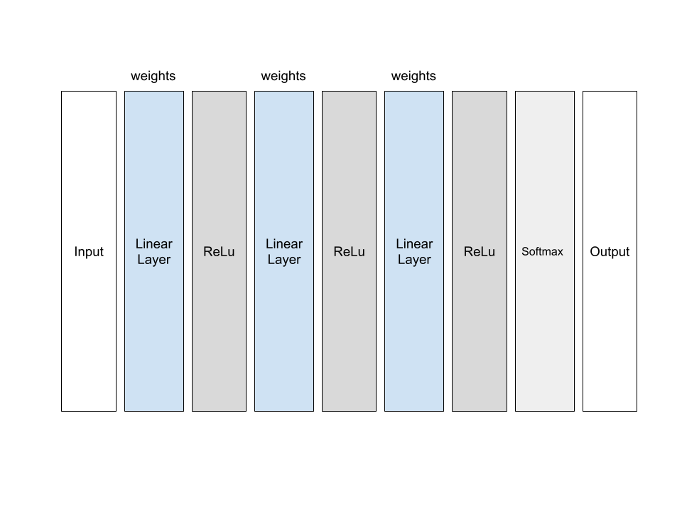
The neural net is an 8,643 parameter model containing 5 layers: the input layer (100), three hidden layers (64, 32, 3), and the softmax output layer. Each layer has weight matrix , and each layer is fully connected. In this case, we determined experimentally that the width of each layer has more impact on training accuracy than the number of layers, hence why it’s shallow.
| Epoch | Training accuracy | Test accuracy |
|---|---|---|
| 10 | 99.00% | 97.5% |
| 20 | 99.62% | 98.37% |
| 30 | 99.80% | 98.53% |
| 40 | 99.77% | 98.07% |
| 50 | 99.81% | 98.53% |
So we can see that the model roughly converged in the first 10 epochs. This is a very simple example (that can easily fit on an STM32). We can also see that the problem is too simple, given that it converged so quickly.